Casio CFX-9850G PLUS Graphing Manual

Brand: Casio

Model: CFX-9850G PLUS

Type: Graphing Manual

This manual is also suitable for

Graphing

A collection of versatile graphing tools plus a large 127 × 63-dot

display makes it easy to draw a variety of function graphs quickly

and easily. This calculator is capable of drawing the following

types of graphs.

•Rectangular coordinate (Y =) graphs

•Polar coordinate (r =) graphs

•Parametric graphs

•X = constant graphs

•Inequality graphs

•Integration graphs (in the RUN mode only)

A selection of graph commands also makes it possible to incor-

porate graphing into programs.

8-1 Before Trying to Draw a Graph

8-2 View Window (V-Window) Settings

8-3 Graph Function Operations

8-4 Graph Memory

8-5 Drawing Graphs Manually

8-6 Other Graphing Functions

8-7 Picture Memory

8-8 Graph Background

Chapter

112

8-1 Before Trying to Draw a Graph

k Entering the Graph Mode

On the Main Menu, select the GRAPH icon and enter the GRAPH Mode. When

you do, the Graph Function menu appears on the display. You can use this menu

to store, edit, and recall functions and to draw their graphs.

• {SEL} ... {draw/non-draw status}

• {DEL} ... {function delete}

• {TYPE} ... {graph type menu}

• {COLR} ... {graph color}

• {GMEM} ... {graph memory save/recall}

• {DRAW} ... {graph draw}

Memory area

Use

and

to change selection.

CFX

113

8-2 View Window (V-Window) Settings

Use the View Window to specify the range of the x-and y-axes, and to set the

spacing between the increments on each axis. You should always set the View

Window parameters you want to use before drawing a graph.

1. Press !3(V·Window) to display

the View Window.

X min ............ Minimum x-axis value

X max ........... Maximum x-axis value

X scale ......... Spacing of x-axis increments

Y min ............ Minimum y-axis value

Y max ........... Maximum y-axis value

Y scale .......... Spacing of y-axis increments

• {INIT}/{TRIG}/{STD} ... View Window {initial settings}/{initial settings using

specified angle unit}/{standardized settings}

• {STO}/{RCL} ... View Window setting {store}/{recall}

The nearby illustration shows the meaning

of each of these parameters.

2. Input a value for a parameter and press w. The calculator automatically

selects the next parameter for input.

•You can also select a parameter using the c and f keys.

• There are actually nine View Window parameters. The remaining three

parameters appear on the display when you move the highlighting down past

the Y scale parameter by inputting values and pressing c.

min .......... T,

minimum values

max ......... T,

maximum values

pitch ........ T,

pitch

P. 115

P. 116

X min

X scale

Y min

Y max

X max

Y scale

(x, y)

114

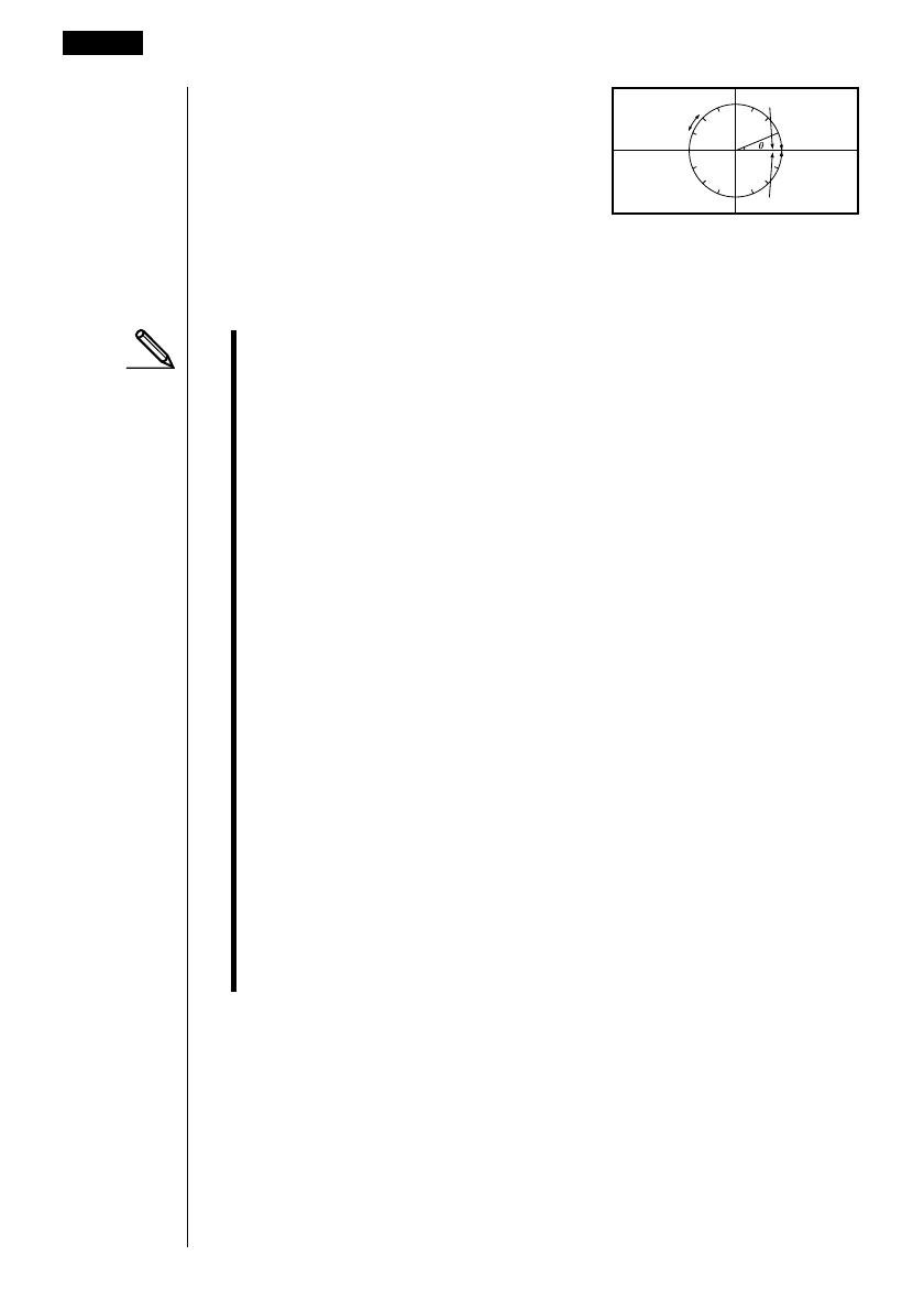
The nearby illustration shows the meaning

of each of these parameters.

3. To exit the View Window, press J or ! Q.

•Pressing w without inputting any value also exits the View Window.

• The following is the input range for View Window parameters.

–9.9999E+97 to 9.99999E+97

•You can input parameter values up to 14 digits long. Values greater than 10

or less than 10

-2

, are automatically converted to a 7-digit mantissa (including

negative sign) plus a 2-digit exponent.

• The only keys that enabled while the View Window is on the display are: a

to j, ., E, -, f, c, d, e, +, -, *, /, (, ), ! 7,

J, ! Q. You can use - or - to input negative values.

• The existing value remains unchanged if you input a value outside the

allowable range or in the case of illegal input (negative sign only without a

value).

•Inputting a View Window range so the min value is greater than the max

value, causes the axis to be inverted.

•You can input expressions (such as 2π) as View Window parameters.

•When the View Window setting does not allow display of the axes, the scale

for the y-axis is indicated on either the left or right edge of the display, while

that for the x-axis is indicated on either the top or bottom edge.

•When View Window values are changed, the graph display is cleared and the

newly set axes only are displayed.

•View Window settings may cause irregular scale spacing.

•Setting maximum and minimum values that create too wide of a View

Window range can result in a graph made up of disconnected lines (because

portions of the graph run off the screen), or in graphs that are inaccurate.

• The point of deflection sometimes exceeds the capabilities of the display with

graphs that change drastically as they approach the point of deflection.

•Setting maximum and minimum values that create to narrow of a View

Window range can result in an error.

8 - 2 View Window (V-Window) Settings

)

(

X, Y

)

min

max

pitch

115

k Initializing and Standardizing the View Window

uTo initialize the View Window

You can use either of the following two methods to initialize the View Window.

Normal initialization

Press !3 (V-Window) 1 (INIT) to initialize the View Window to the following

settings.

Xmin = –6.3 Ymin = –3.1

Xmax = 6.3 Ymax = 3.1

Xscale = 1 Yscale = 1

Trigonometric initialization

Press ! 3 (V-Window) 2 (TRIG) to initialize the View Window to the

following settings.

Deg Mode

Xmin = –540 Ymin = –1.6

Xmax = 540 Ymax = 1.6

Xscale = 90 Yscale = 0.5

Rad Mode

Xmin = –9.4247779

Xmax = 9.42477796

Xscale = 1.57079632

Gra Mode

Xmin = –600

Xmax = 600

Xscale = 100

• The settings for Y min, Y max, Y pitch, T/

min, T/

max, and T/

pitch remain

unchanged when you press 2 (TRIG).

uTo standardize the View Window

Press !3 (V-Window) 3 (STD) to standardize the View Window to the

following settings.

Xmin = –10 Ymin = –10

Xmax = 10 Ymax = 10

Xscale = 1 Yscale = 1

View Window (V-Window) Settings 8 - 2

116

8 - 2 View Window (V-Window) Settings

k View Window Memory

You can store up to six sets of View Window settings in View Window memory for

recall when you need them.

uTo store View Window settings

Inputting View Window values and then pressing 4 (STO) 1 (V·W1) stores the

View Window contents in View Window memory V·W1.

• There are six View Window memories numbered V·W1 to V·W6.

•Storing View Window settings in a memory area that already contains settings

replaces the existing settings with the new ones.

uTo recall View Window settings

Pressing 5 (RCL) 1 (V·W1) recalls the contents of View Window memory

V·W1.

•Recalling View Window settings causes the settings currently on the display to

be deleted.

•You can change View Window settings in a program using the following

syntax.

View Window [X min value], [X max value], [X scale value],

[Y min value], [Y max value], [Y scale value],

[T,

min value], [T,

max value], [T,

pitch value]

117

8-3 Graph Function Operations

You can store up to 20 functions in memory. Functions in memory can be edited,

recalled, and graphed.

k Specifying the Graph Type

Before you can store a graph function in memory, you must first specify its graph

type.

1. While the Graph Function Menu is on the display, press 3 (TYPE) to display

the graph type menu, which contains the following items.

•{Y=}/{r=}/{Parm}/{X=c} ... {rectangular coordinate}/{polar coordinate}/

{parametric}/{X=constant} graph

•{Y>}/{Y<}/{Y

t}/{Y

s} ... {Y>f(x)}/{Y<f(x)}/{Y>f(x)}/{Y<f(x)} inequality graph

2. Press the function key that corresponds to the graph type you want to specify.

k Storing Graph Functions

uTo store a rectangular coordinate function (Y =)

Example To store the following expression in memory area Y1 :

y = 2 x

– 5

3(TYPE)1(Y =) (Specifies rectangular coordinate expression.)

cvx-f(Inputs expression.)

w (Stores expression.)

•You will not be able to store the expression in an area that already contains a

parametric function. Select another area to store your expression or delete the

existing parametric function first. This also applies when storing r = expres-

sions, X = constant expressions, and ineqalities.

uTo store a polar coordinate function (r =)

Example To store the following expression in memory area r2 :

r = 5 sin 3

3(TYPE)2(r =) (Specifies polar coordinate expression.)

fsdv(Inputs expression.)

w(Stores expression.)

118

uTo store a parametric function

Example To store the following functions in memory areas Xt3 and Yt3 :

x = 3 sin T

y = 3 cos T

3(TYPE)3(Parm) (Specifies parametric expression.)

dsvw(Inputs and stores x expression.)

dcvw(Inputs and stores y expression.)

•You will not be able to store the expression in an area that already contains a

rectangular coordinate expression, polar coordinate expression, X = constant

expression or inequality. Select another area to store your expression or delete

the existing expression first.

uTo store an X = constant expression

Example To store the following expression in memory area X4 :

X = 3

3(TYPE)4(X = c) (Specifies X = constant expression.)

d(Inputs expression.)

w(Stores expression.)

•Inputting X, Y, T, r, or

for the constant in the above procedures causes an

error.

uTo store an inequality

Example To store the following inequality in memory area Y5 :

y > x

– 2x – 6

3(TYPE)6(g)1(Y>) (Specifies an inequality.)

vx-cv-g(Inputs expression.)

w(Stores expression.)

8 - 3 Graph Function Operations

119

k Editing Functions in Memory

uTo edit a function in memory

Example To change the expression in memory area Y1 from y = 2x

– 5

to y = 2x

– 3

e (Displays cursor.)

eeeed(Changes contents.)

w(Stores new graph function.)

uTo delete a function

1. While the Graph Function Menu is on the display, press f or c to display

the cursor and move the highlighting to the area that contains the function you

want to delete.

2. Press 2 (DEL).

3. Press 1 (YES) to delete the function or 6 (NO) to abort the procedure

without deleting anything.

Parametric functions come in pairs (Xt and Yt).

When editing a parametric function, clear the graph functions and re-input from

the beginning.

k Drawing a Graph

uTo specify the graph color

The default color for graph drawing is blue, but you can change the color to

orange or green if you want.

1. While the Graph Function Menu is on the display, press f or c to display

the cursor and move the highlighting to the area that contains the function

whose graph color you want to change.

2. Press 4 (COLR) to display a color menu, which contains the following items.

• {Blue}/{Orng}/{Grn} ... {blue}/{orange}/{green}

3. Press the function key for the color you want to use.

Graph Function Operations 8 - 3

CFX

120

uTo specify the draw/non-draw status of a graph

Example To select the following functions for drawing :

Y1 = 2x

– 5 r2 = 5 sin3

Use the following View Window parameters.

Xmin = –5 Ymin = –5

Xmax = 5 Ymax = 5

Xscale = 1 Yscale = 1

(Select a memory area that contains a

function for which you want to specify

non-draw.)

1(SEL)

(Specify non-draw.)

cc1(SEL)

c1(SEL)

6(DRAW) or w

(Draws the graphs.)

•Pressing ! 6 (G↔T) or A returns to the Graph Function Menu.

8 - 3 Graph Function Operations

Unhighlights

121

•You can use the set up screen settings to alter the appearance of the graph

screen as shown below.

•Grid: On (Axes: On Label: Off)

This setting causes dots to appear at the grid intersects on the display.

•Axes: Off (Label: Off Grid: Off)

This setting clears the axis lines from the display.

• Label: On (Axes: On Grid: Off)

This setting displays labels for the x- and y-axes.

•A polar coordinate (r =) or parametric graph will appear coarse if the settings

you make in the View Window cause the T,

pitch value to be too large,

relative to the differential between the T,

min and T,

max settings. If the

settings you make cause the T,

pitch value to be too small relative to the

differential between the T,

min and T,

max settings, on the other hand, the

graph will take a very long time to draw.

•Attempting to draw a graph for an expression in which X is input for an X =

constant expression results in an error.

Graph Function Operations 8 - 3

P. 6

122

Graph Function Operations 8 - 3

8-4 Graph Memory

Graph memory lets you store up to six sets of graph function data and recall it

later when you need it.

A single save operation saves the following data in graph memory.

•All graph functions in the currently displayed Graph Function Menu (up to 20)

•Graph types

•Graph colors

•Draw/non-draw status

•View Window settings (1 set)

uTo store graph functions in graph memory

Pressing 5(GMEM) 1(STO) 1(GM1) stores the selected graph function into

graph memory GM1.

• There are six graph memories numbered GM1 to GM6.

•Storing a function in a memory area that already contains a function replaces

the existing function with the new one.

• If the data exceeds the calculator’s remaining memory capacity, an error

occurs.

uTo recall a graph function

Pressing 5 (GMEM) 2 (RCL) 1 (GM1) recalls the contents of graph memory

GM1.

•Recalling data from graph memory causes any data currently on the Graph

Function Menu to be deleted.

CFX

123

8-5 Drawing Graphs Manually

After you select the RUN icon in the Main Menu and enter the RUN Mode, you

can draw graphs manually. First press ! 4 (Sketch) 5 (GRPH) to recall the

Graph Command Menu, and then input the graph function.

• {Y=}/{r=}/{Parm}/{X=c}/{G∫dx} ... {rectangular coordinate}/{polar coordinate}/

{parametric}/{X = constant}/{integration} graph

• {Y>}/{Y<}/{Y

t}/{Y

s} ... {Y>f(x)}/{Y<f(x)}/{Y>f(x)}/{Y<f(x)} inequality graph

uTo graph using rectangular coordinates (Y =) [Sketch]-[GRPH]-[Y=]

You can graph functions that can be expressed in the format y = f(x).

Example To graph y = 2x

+ 3x – 4

Use the following View Window parameters.

Xmin = –5 Ymin = –10

Xmax = 5 Ymax = 10

Xscale = 2 Yscale = 5

1. In the set up screen, specify “Y=” for Func Type and then press J.

2. Input the rectangular coordinate (Y =) expression.

!4(Sketch)1(Cls)w

5(GRPH)1(Y =) cvx+dv-e

3. Press w to draw the graph.

•You can draw graphs of the following built-in scientific functions.

• sin x • cos x • tan x • sin

–1

x • cos

–1

• tan

–1

x • sinh x • cosh x • tanh x • sinh

–1

• cosh

–1

x • tanh

–1

x • • x

• log x

• lnx • 10

• e

• x

–1

•

View Window settings are made automatically for built-in graphs.

124

uTo graph using polar coordinates (

r =) [Sketch]-[GRPH]-[r=]

You can graph functions that can be expressed in the format

r = f

(

Example To graph r = 2 sin3

Use the following View Window parameters.

Xmin = –3 Ymin = –2 T,

min = 0

Xmax = 3 Ymax = 2 T,

max = π

Xscale = 1 Yscale = 1 T,

pitch = π÷36

1. In the set up screen, specify “r =” for Func Type.

2. Specify “Rad” as the angle unit and then press J.

3. Input the polar coordinate expression (r =).

!4(Sketch)1(Cls)w

5(GRPH)2(r =)csdv

4. Press w to draw the graph.

•You can draw graphs of the following built-in scientific functions.

• sin

• cos

• tan

• sin

–1

• cos

–1

• tan

–1

• sinh

• cosh

• tanh

• sinh

–1

• cosh

–1

• tanh

–1

•

• log

• ln

• 10

• e

•

–1

•

View Window settings are made automatically for built-in graphs.

8 - 5 Drawing Graphs Manually

125

uTo graph parametric functions

[Sketch]-[GRPH]-[Parm]

You can graph parametric functions that can be expressed in the following format.

(X, Y) = (

f (T), g (T))

Example To graph the following parametric functions:

x = 7 cos T – 2 cos 3.5T y = 7 sin T – 2 sin 3.5T

Use the following View Window parameters.

Xmin = –20 Ymin = –12 T,

min = 0

Xmax = 20 Ymax = 12 T,

max = 4π

Xscale = 5 Yscale = 5 T,

pitch = π÷36

1. In the set up screen, specify “Parm” for Func Type.

2. Specify “Rad” (radians) as the angle unit and then press J.

3. Input the parametric functions.

!4(Sketch)1(Cls)w

5(GRPH)3(Parm)

hcv-ccd.fv,

hsv-csd.fv)

4. Press w to draw the graph.

uTo graph X = constant [Sketch]-[GRPH]-[X=c]

You can graph functions that can be expressed in the format X = constant.

Example To graph X = 3

Use the following View Window parameters.

Xmin = –5 Ymin = –5

Xmax = 5 Ymax = 5

Xscale = 1 Yscale = 1

1. In the set up screen, specify “X=c” for Func Type and then press J.

Drawing Graphs Manually 8 - 5

126

2. Input the expression.

!4(Sketch)1(Cls)w

5(GRPH)4(X = c)d

3. Press w to draw the graph.

uTo graph inequalities [Sketch]-[GRPH]-[Y>]/[Y<]/[Y≥]/[Y≤]

You can graph inequalities that can be expressed in the following four formats.

• y > f

(x)• y < f

(x)• y > f

(x)• y < f

(x)

Example To graph the inequality y > x

– 2x – 6

Use the following View Window parameters.

Xmin = –6 Ymin = –10

Xmax = 6 Ymax = 10

Xscale = 1 Yscale = 5

1. In the set up screen, specify “Y>” for Func Type and then press J.

2. Input the inequality.

!4(Sketch)1(Cls)w

5(GRPH)6(g) 1(Y>)vx-cv-g

3. Press w to draw the graph.

8 - 5 Drawing Graphs Manually

127

uTo draw an integration graph

[Sketch]-[GRPH]-[G∫dx]

You can graph an integration calculation performed using the function

y = f(x).

Example To graph the following, with a tolerance of “tol” = 1E - 4:

∫

–2

(x + 2) (x – 1) (x – 3) dx

Use the following View Window parameters.

Xmin = –4 Ymin = –8

Xmax = 4 Ymax = 12

Xscale = 1 Yscale = 5

1. In the set up screen, specify “Y=” for Func Type and then press J .

2. Input the integration graph expression.

!4(Sketch)1(Cls)w

5(GRPH)5(G∫dx)(v+c)(v-b)

(v-d),-c,b,bE-e

3. Press w to draw the graph.

•Before drawing an integration graph, be sure to always press ! 4 (Sketch)

1 (Cls) to clear the screen.

•You can also incorporate an integration graph command into programs.

Drawing Graphs Manually 8 - 5

128

8-6 Other Graphing Functions

The functions described in this section tell you how to read the x- and y-coordi-

nates at a given point, and how to zoom in and zoom out on a graph.

• These functions can be used with rectangular coordinate, polar coordinate,

parametric, X = constant, and inequality graphs only.

k Connect Type and Plot Type Graphs (Draw Type)

You can use the Draw Type setting of the set up screen to specify one of two

graph types.

•Connect

Points are plotted and connected by lines to create a curve.

•Plot

Points are plotted without being connected.

k Trace

With trace, you can move a flashing pointer along a graph with the cursor keys

and obtain readouts of coordinates at each point. The following shows the different

types of coordinate readouts produced by trace.

•Rectangular Coordinate Graph • Polar Coordinate Graph

•Parametric Function Graph • X = Constant Graph

•Inequality Graph

uTo use trace to read coordinates

Example To determine the points of intersection for graphs produced by

the following functions:

Y1 = x

– 3 Y2 = –x + 2

Use the following View Window parameters.

Xmin = –5 Ymin = –10

Xmax = 5 Ymax = 10

Xscale = 1 Yscale = 2

P. 5

129

1. After drawing the graphs, press 1 (Trace) to display the pointer in the center

of the graph.

• The pointer may not be visible on the graph

when you press 1 (Trace).

2. Use d to move the pointer to the first intersection.

d ~ d

•Pressing d and e moves the pointer along the graph. Holding down either

key moves the pointer at high speed.

3. Use f and c to move the pointer between the two graphs.

4. Use e to move the pointer to the other intersection.

e ~ e

•To abort a trace operation, press 1 (Trace).

•Do not press the A key while performing a trace operation.

uTo display the derivative

If the Derivative item in the set up screen is set to “On”, the derivative appears on

the display along with the coordinate values.

x/y

coordinate values

Other Graphing Functions 8 - 6

P. 5

130

• The following shows how the display of coordinates and the derivative changes

according to the Graph Type setting.

•Rectangular Coordinate Graph • Polar Coordinate Graph

•Parametric Function Graph • X = Constant Graph

•Inequality Graph

• The derivative is not displayed when you use trace with a built-in scientific

function.

•Setting the Coord item in the set up screen to “Off” turns display of the

coordinates for the current pointer location off.

uScrolling

When the graph you are tracing runs off the display along either the x- or y-axis,

pressing the e or d cursor key causes the screen to scroll in the correspond-

ing direction eight dots.

•You can scroll only rectangular coordinate and inequality graphs while tracing.

You cannot scroll polar coordinate graphs, parametric function graphs, or X =

constant graphs.

• The graph on the screen does not scroll when you are tracing while the Dual

Screen Mode is set to “Graph” or “G to T”.

•Trace can be used only immediately after a graph is drawn. It cannot be used

after changing the settings of a graph.

• The x- and y-coordinate values at the bottom of the screen are displayed

using a 12-digit mantissa or a 7-digit mantissa with a 2-digit exponent. The

derivative is displayed using a 6-digit mantissa.

•You cannot incorporate trace into a program.

•You can use trace on a graph that was drawn as the result of an output

command (^), which is indicated by the “-Disp-” indicator on the screen.

k Scroll

You can scroll a graph along its x- or y-axis. Each time you press f, c, d, or

e, the graph scrolls 12 dots in the corresponding direction.

8 - 6 Other Graphing Functions

P. 6

P. 7

Page is loading ...

Casio CFX-9850G PLUS Graphing Manual

Brand: Casio

Model: CFX-9850G PLUS

Type: Graphing Manual

This manual is also suitable for

Download PDF

report

Casio CFX-9850G PLUS Graphing Manual

This manual is also suitable for

Casio CFX-9850G PLUS Graphing Manual

Related papers

Other documents